Notebook 5 - Sound
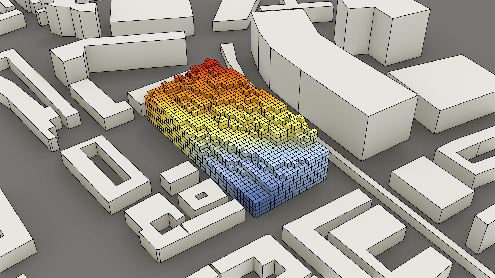
The following conducts a sound analysis for each voxel in the building. While the script does produce the desired result it is not entirely physically correct.
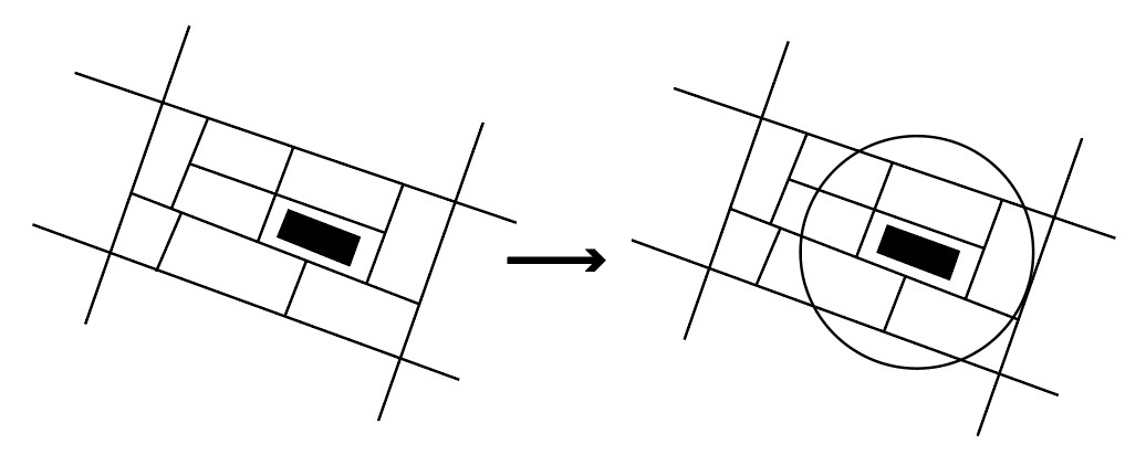
The first step in the script is to import the roads with different sound values as separate lists. The road map used for this calculation was made by hand based on intuition. The loudness of the different road types were estimated with an online tool. The next step is to select a radius around the envelope for analysis. This radius should be large enough for an accurate calculation but should not be too large to keep it computationally viable.
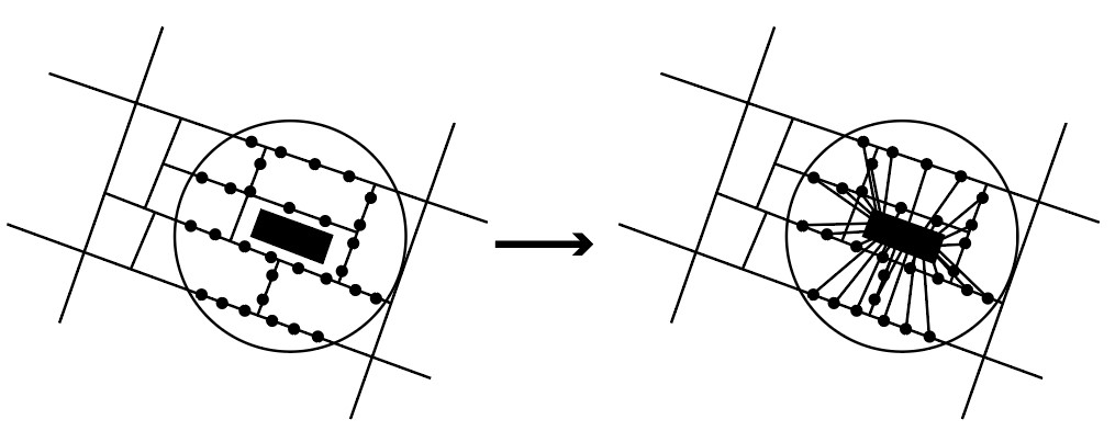
The roads within this radius are then divided into points and the distance is measured from each voxel to each point. We use the rule of dB lowers by 6 when the distance to the source doubles. After this step, we stray from accurate physics and use a mass addition to calculate the noise for each voxel. In real life, noise cannot just be added to each other. We however chose this approach to keep the analysis simple and within our reach.
To forego the computational limitations of grasshopper we split the calculation for each level of the building. This prevents crashes and allows us to get a more defined calculation overall.
The data per floor is pickled and saved in data/sound.
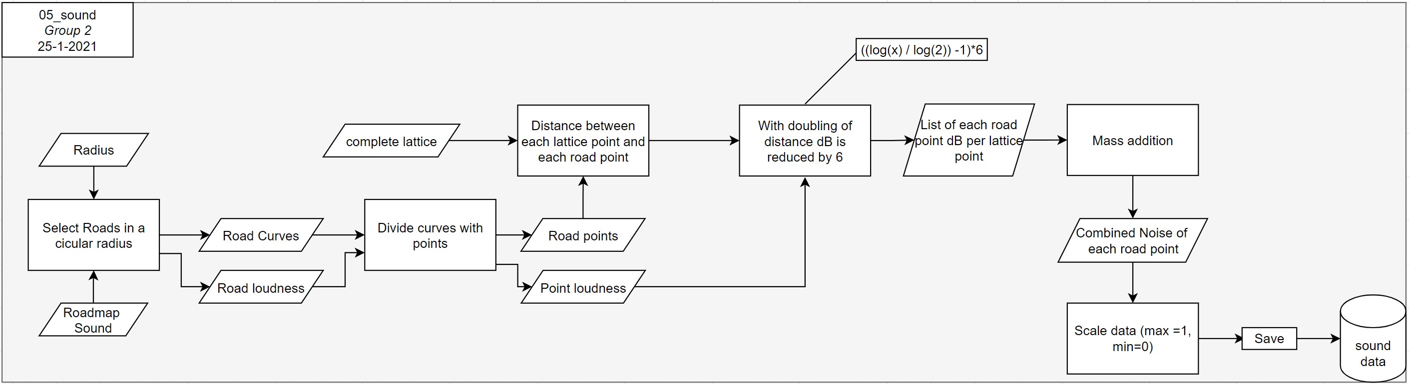
Flowchart
The flowchart as shown in Figure 40 is in the second (blue) section of the fundamental flowchart as shown in the Planning - products.
Additional diagrams
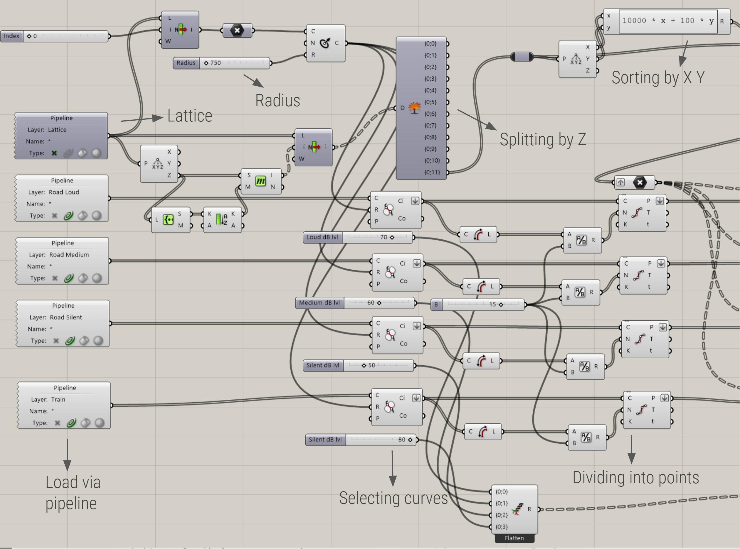
Figure 41 shows the grasshopper schript of the first steps in which the curves are loaded and picked within radius.
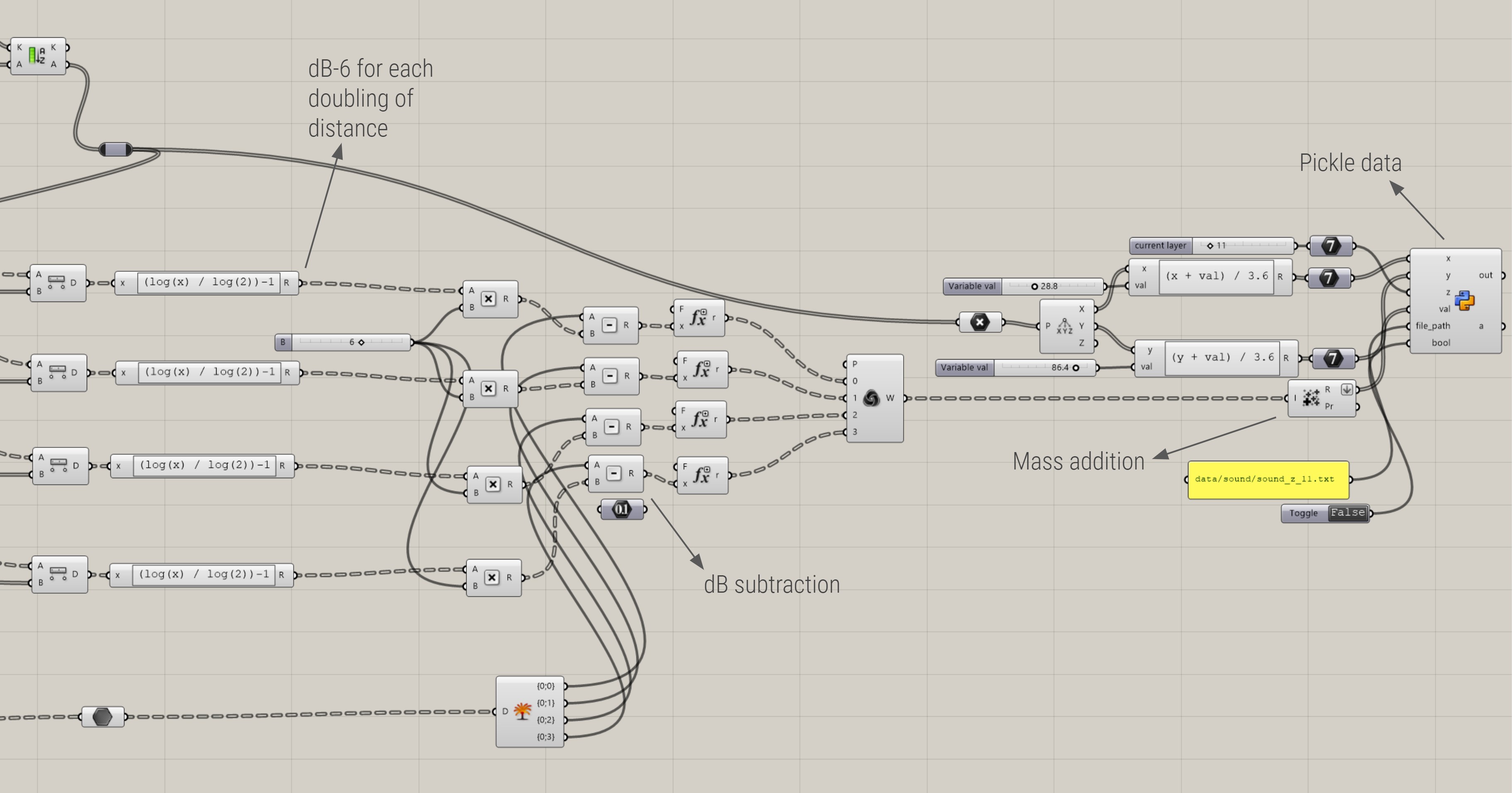
In Figure 42, grasshopper file for the last part of the script in which the calculation is done and the data exported, is visualized
A visualisation of the first step of establishing the radius is shown in Figure 43
After that, the curves are divided and distances are measured, as you can see in Figure 44.
Pseudo code
For a better understanding of the code, we wrote a pseudo code. Grasshopper file 5, and the other notebooks, can be found here.
For coordinates in center cluster
    add a center next to the center in the x direction

Stack the centers vertically
Add all centers in cluster final list

For cluster center in cluster final
    set 1 in shaft lattice
Assign maximum height for the shafts

#Creation of horizontal corridors
Take the stencil, lattice and adress of a voxel in that lattice
Returns the indices of the neigbhours of that voxel
Find the number of all voxels
Initialize the adjacency matrix
Find the index of the available voxels in availability lattice
Fill the adjacency matrix using the list of all neigbhours

For voxel location in availability index
  Find the 1 dimensional id
  Retrieve the list of neighbours of the voxels based on the stencil

  For neighbours in voxel neighbours
      Set the entry to 1

Construct the graph

#Find the shortest path to the cluster centres seeds and construct the corridor
Define the clusters again
Initialize corridor lattice

For each voxel that needs to have access to shafts
  For available voxel in occupation index cluster
    Slice the corridor lattice horizontally
    Find the vertical shaft voxel indices
    Construct the destination address
    Construct 1-dimensional indices
      Try
        Find the shortest path
        Set the shortest path as occupied in the coordinate flat path = 1
    Except
        Print "unreachable" when the voxel is unreachable

Reshape the flat lattice
Visualisations of the result
GIF
Voxelcloud